Make hexagon maps

Skills learned

Use this page to:

Create hexagonal grids to summarize dominant LANFDIRE vegetation types across example landscape, enabling spatial analysis beyond raster cell comparisons
Build an interactive Leaflet map with toggle display to visualize dominant BpS and EVT within each hexagon

Set up

For this work we will use the Area of Interest shapefile, and pre-downloaded BpS and EVT rasters. Before you can complete this page you will need to complete the work on the Download data and Prepare rasters pages.

Code to load packages and inputs

# Load packages
library(exactextractr)
library(jsonlite)
library(leaflet)
library(leaflet.providers)
library(RColorBrewer)
library(sf)
library(terra)
library(tidyverse)


# read in Area of Interest (aoi) shapefile

shp <- st_read("inputs/map_zone_35.shp", quiet = TRUE) %>% 
  st_transform(crs = 5070) %>%
  st_union() %>%
  st_sf()

# read in .csv of CONUS-wide attributes for later joining to AoI BpS table

bps_conus_atts <- read_csv("inputs/LF20_BPS_220.csv")

# another way is directly from landfire.gov
# bps_url <- "https://landfire.gov/sites/default/files/CSV/LF2016/LF16_BPS.csv" # will likely get warning, but it's OK
# bps_conus_atts <- read.csv(bps_url)


evt_conus_atts <- read_csv("inputs/LF23_EVT_240.csv")

# evt_url <- "https://landfire.gov/sites/default/files/CSV/2024/LF2024_EVT.csv" # will likely get warning, but it's OK
# evt_conus_atts <- read.csv(evt_url)

# load in landfire stacked raster
stacked_rasters <- rast("inputs/landfire_data.tif")

# "split" cropped and masked stacked raster into separate layers
for(lyr in names(stacked_rasters)) assign(lyr, stacked_rasters[[lyr]])

Make hexgrid ~ 25,000 acres a piece

In this step we make a hexgrid map for our area of interest and confirm hexagon size.

# Hexagon side length in meters for ~25,000 ac hexagons
hex_side <- 10930

# Create full hex grid
hex_grid <- st_make_grid(shp,
                         cellsize = hex_side,
                         square = FALSE,
                         what = "polygons") %>%
                          st_sf()

hex_grid_clipped <- st_intersection(hex_grid, shp) %>%
  mutate(index = row_number())


plot(st_geometry(hex_grid_clipped))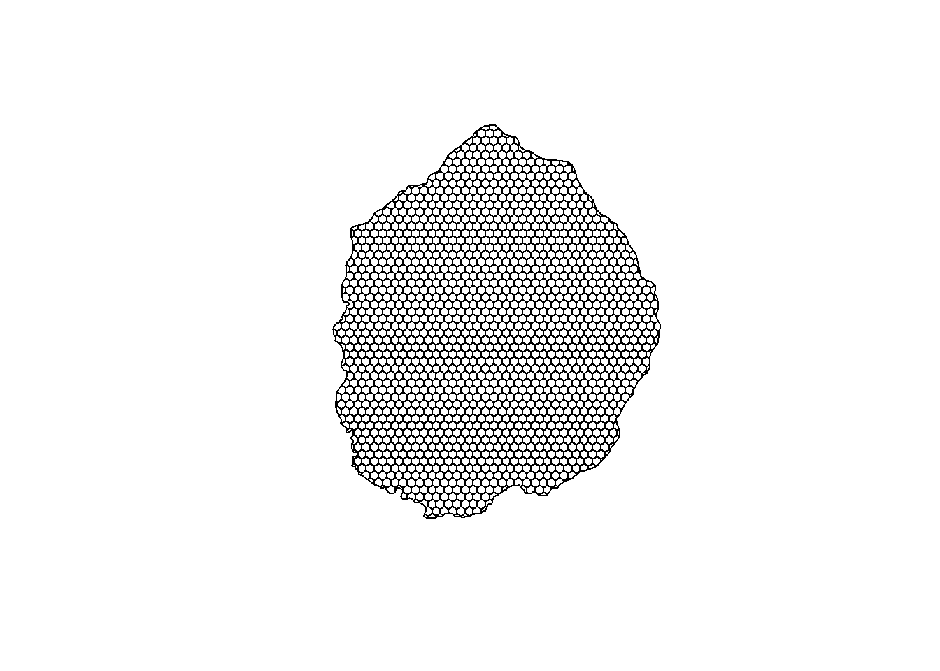

# Calculate area in square meters
hex_grid_size <- hex_grid %>%
  mutate(area_m2 = st_area(.),
         area_acres = as.numeric(area_m2) / 4046.86)

Calculate majority type per hexagon

Below we use the extactextractr package to extract the majority (most dominant) BpS value and EVT value per hexagon, the we join in a minimal number of attributes (e.g., EVT_NAME) for mapping demo.

# bps
bps_majority_hex <- exact_extract(US_200BPS, hex_grid_clipped, 'majority', append_cols = "index") %>%
  left_join(select(bps_conus_atts,
                   VALUE,
                   BPS_MODEL,
                   BPS_NAME,
                   FRI_ALLFIR),
            by = c('majority' = 'VALUE'))

# evt
evt_majority_hex <- exact_extract(US_240EVT, hex_grid_clipped, 'majority', append_cols = "index") %>%
  left_join(select(evt_conus_atts,
                   VALUE,
                   EVT_NAME,
                   EVT_PHYS),
            by = c('majority' = 'VALUE'))

# Join both BpS and EVT attributes to hex shapefile
hexs_bps_evt <- hex_grid_clipped %>%
  left_join(bps_majority_hex, by = 'index') %>%
  left_join(evt_majority_hex, by = 'index')


# save the shapefile for mapping in non-R applications or to read back into R

st_write(hexs_bps_evt, "outputs/bps_evt_hexs.shp")

Make the map

Below we use our attributed hexgrid to make a clickable leaflet map with the BpS and EVT layers for our area of interest.

hexs_bps_evt <- st_read("outputs/bps_evt_hexs.shp")

Reading layer `bps_evt_hexs' from data source 
  `C:\Users\rswaty\Documents\r_demos\outputs\bps_evt_hexs.shp' 
  using driver `ESRI Shapefile'
Simple feature collection with 1648 features and 8 fields
Geometry type: MULTIPOLYGON
Dimension:     XY
Bounding box:  xmin: -508742.8 ymin: 655736 xmax: -74984.26 ymax: 1177230
Projected CRS: NAD83 / Conus Albers

hexs_bps_evt <- st_transform(hexs_bps_evt , crs = 4326)

# Create a dynamic color palette
bps_names <- unique(hexs_bps_evt$BPS_NAME)
evt_names <- unique(hexs_bps_evt$EVT_NAME)

# Use a colorblind-friendly base palette and expand it
base_palette <- RColorBrewer::brewer.pal(8, "Set2")  # Set2 is colorblind-friendly
bps_colors <- colorRampPalette(base_palette)(length(bps_names))

pal_bps <- colorFactor(
  palette = bps_colors,
  domain = bps_names
)

# Repeat for EVT
evt_colors <- colorRampPalette(base_palette)(length(evt_names))

pal_evt <- colorFactor(
  palette = evt_colors,
  domain = evt_names
)




# Get the bounding box of the shapefile
bbox <- st_bbox(hexs_bps_evt)

# Convert bounding box to named list
bbox_list <- as.list(bbox)

# Convert named list to JSON
json_output <- toJSON(bbox_list, keep_vec_names = TRUE)



leaflet(hexs_bps_evt) %>%
  addTiles() %>%

  fitBounds(lng1 = bbox_list$xmin, lat1 = bbox_list$ymin, lng2 = bbox_list$xmax, lat2 = bbox_list$ymax) %>%

  addPolygons(
    fillColor = ~pal_bps(BPS_NAME),
    color = "#BDBDC3",
    weight = 1,
    opacity = 1,
    fillOpacity = 1.0,
    highlightOptions = highlightOptions(
      weight = 2,
      color = "#666",
      fillOpacity = 1.0,
      bringToFront = TRUE
    ),
    label = ~BPS_NAME,
    labelOptions = labelOptions(
      style = list("font-weight" = "normal", padding = "3px 8px"),
      textsize = "15px",
      direction = "auto"
    ),
    group = "Biophysical Settings"
  ) %>%
  addPolygons(
    fillColor = ~pal_evt(EVT_NAME),
    color = "#BDBDC3",
    weight = 1,
    opacity = 1,
    fillOpacity = 1.0,
    highlightOptions = highlightOptions(
      weight = 2,
      color = "#666",
      fillOpacity = 1.0,
      bringToFront = TRUE
    ),
    label = ~EVT_NAME,
    labelOptions = labelOptions(
      style = list("font-weight" = "normal", padding = "3px 8px"),
      textsize = "15px",
      direction = "auto"
    ),
    group = "Existing Vegetation Types"
  ) %>%
addLayersControl(
    overlayGroups = c("Biophysical Settings", "Existing Vegetation Types"),
    options = layersControlOptions(collapsed = FALSE)
  ) %>%
  hideGroup("Existing Vegetation Types") %>% # Hide this group initially
  addScaleBar(position = "bottomleft", options = scaleBarOptions(metric = TRUE, imperial = FALSE))