Make charts with LANDFIRE data

Skills learned

Use this page to:

Practice summarizing LANDFIRE Biophysical Settings data using R to identify dominant vegetation types across the example landscape
Create bar charts to visualize relative percentages and acerage, gaining experience in data grouping, plotting, and interpretation

Set up

To run the code below you will need to:

Work through the preceding pages, Download data and Prepare rasters for your own Area of Interest OR
Make sure you have a datasheet with BpS names and Relative Percentages at the least. We will load in the data for our Area of Interest for you to work with if you do not have your own data.

Code to load packages and inputs, summarize data

# load packages
library(tidyverse)
library(scales)
library(stringr)

# read in data for our Area of Interest
bps_data <- read.csv("outputs/bps_aoi_attributes.csv")
evt_data <- read.csv("outputs/evt_aoi_attributes.csv")

Basic bar chart of the Biophysical Settings

# summarize data by BpS Name attribute for chart.  We do this as an AoI may have multiple variants if it crosses multiple Map Zones. We also limit output dataframe to the top 10 BpSs.  Customize as needed!

bps_name <- bps_data %>%
  group_by(BPS_NAME) %>%
  summarize(ACRES = sum(ACRES),
            REL_PERCENT = sum(REL_PERCENT)) %>%
  arrange(desc(REL_PERCENT)) %>%
  top_n(n = 10, wt = REL_PERCENT)

# plot
bps_percent_chart <- 
  ggplot(data = bps_name, aes(x = BPS_NAME, y = REL_PERCENT)) + 
  geom_bar(stat = "identity") +
  labs(
    title = "Top 10 Biophysical Settings",
    subtitle = "Represents dominant vegetation systems pre-European colonization",
    caption = "Data from landfire.gov.",
    x = "",
    y = "Percent of landscape") +
  scale_x_discrete(limits = rev(bps_name$BPS_NAME),
                   labels = function(x) str_wrap(x, width = 18)) +
  coord_flip() +
  theme_bw(base_size = 14)


bps_acres_chart <-
  ggplot(data = bps_name, aes(x = BPS_NAME, y = ACRES)) + 
  geom_bar(stat = "identity") +
  labs(
    title = "Top 10 Biophysical Settings",
    subtitle = "Represents dominant vegetation systems pre-European colonization",
    caption = "Data from landfire.gov.",
    x = "",
    y = "Acres") +
  scale_x_discrete(limits = rev(bps_name$BPS_NAME),
                   labels = function(x) str_wrap(x, width = 18)) +
  coord_flip() +
  theme_bw(base_size = 14) +
  scale_y_continuous(labels = comma)

bps_acres_chart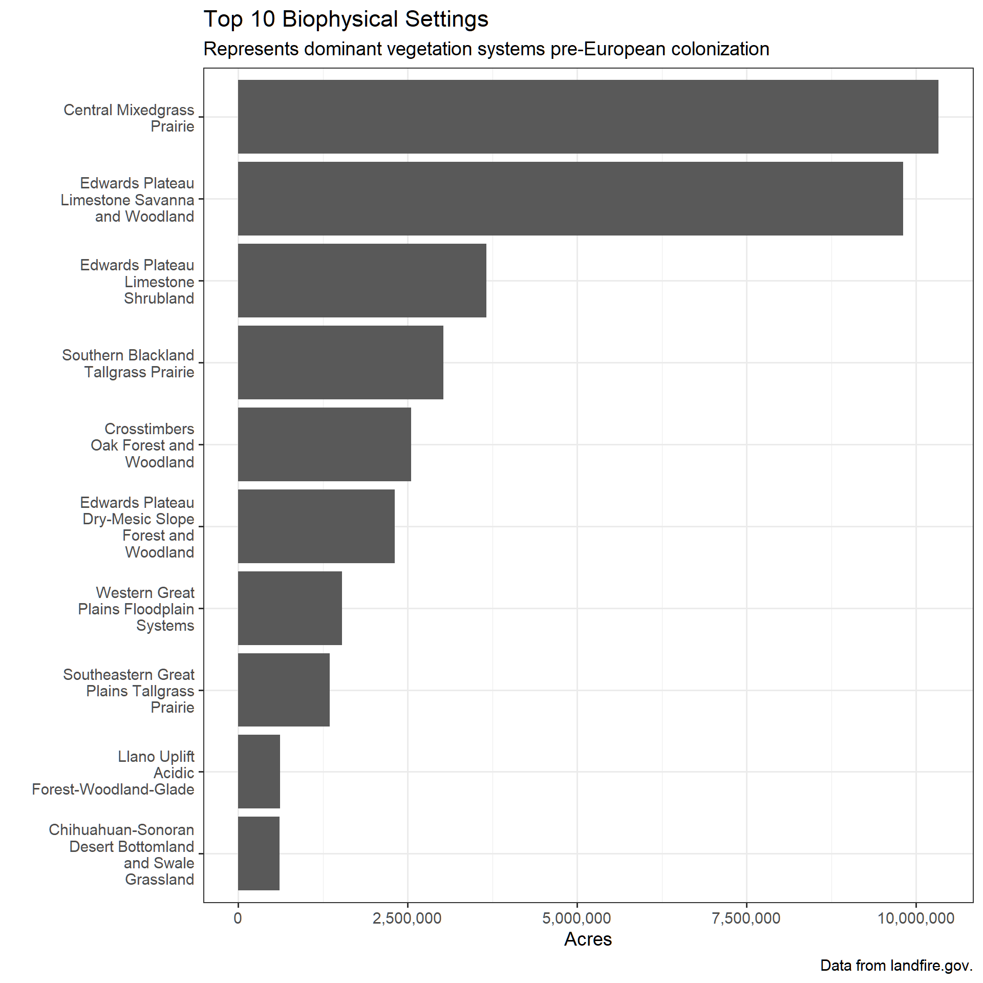

This chart can be easily replicated for the Existing Vegetation Type data by swapping out input data and names in the chart code. Give it a try!

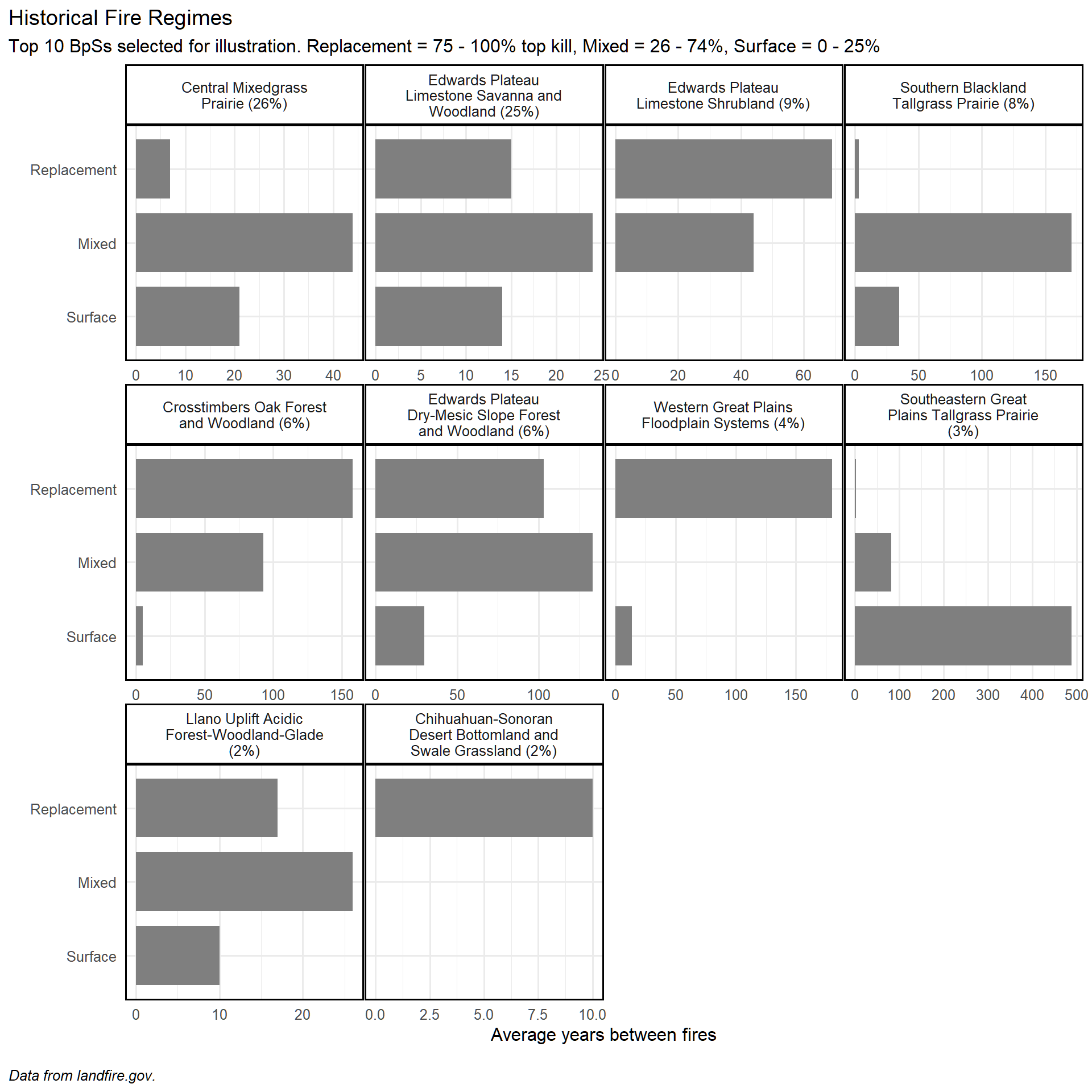
Fire return interval per BpS

# Rename columns for clarity
bps_data_clean <- bps_data %>%
  rename(
    Replacement = FRI_REPLAC,
    Mixed = FRI_MIXED,
    Surface = FRI_SURFAC
  )

# Filter top 10 BPS_NAMEs by REL_PERCENT
top_bps <- bps_data_clean %>%
  arrange(desc(REL_PERCENT)) %>%
  slice_head(n = 10) %>%
  mutate(
    BPS_LABEL = paste0(BPS_NAME, " (", round(REL_PERCENT), "%)")
  )

# Reshape to long format
bps_long <- top_bps %>%
  select(BPS_LABEL, REL_PERCENT, Replacement, Mixed, Surface) %>%
  pivot_longer(cols = c(Replacement, Mixed, Surface),
               names_to = "Fire_Regime",
               values_to = "Years") %>%
  filter(Years >= 0)

# Set order of Fire types
bps_long$Fire_Regime <- factor(bps_long$Fire_Regime, levels = c(
  "Surface",
  "Mixed",
  "Replacement"
))

# Order BPS_LABEL by REL_PERCENT
bps_long$BPS_LABEL <- factor(bps_long$BPS_LABEL,
                             levels = top_bps$BPS_LABEL[order(top_bps$REL_PERCENT, decreasing = TRUE)])

# Plot
 fri_chart <- 
  ggplot(bps_long, aes(x = Years, y = Fire_Regime)) +
  geom_bar(stat = "identity", 
           fill = "grey50",
           width = 0.8, ) +  # grey bars
  facet_wrap(~ BPS_LABEL, 
             scales = "free_x",
             labeller = label_wrap_gen(width = 25), 
             nrow(3)) +
  theme_minimal(base_size = 12) +
  labs(
    title = "Historical Fire Regimes",
    subtitle = "Top 10 BpSs selected for illustration. Replacement = 75 - 100% top kill, Mixed = 26 - 74%, Surface = 0 - 25%",
    caption = "\nData from landfire.gov.",
    x = "Average years between fires",
    y = "") +
  theme(plot.caption = element_text(hjust = 0, face= "italic"), #Default is hjust=1
        plot.title.position = "plot", #NEW parameter. Apply for subtitle too.
        plot.caption.position =  "plot") +
  theme(panel.spacing = unit(.05, "lines"),
        panel.border = element_rect(color = "black", fill = NA, linewidth = 1), 
        strip.background = element_rect(color = "black", linewidth  = 1))

 fri_chart