### SET UP ----


# install.packages("arcgisbinding", repos="https://r.esri.com", type="win.binary")

library(tidyverse)
library(sf)
library(rmapshaper)
library(units)
library(arcgisbinding)


# initialize arc
arc.check_product()

### ANCILLARY DATA ----

# prescribed fire type classification
# NOTE: I made this classification. It is not a LANDFIRE
# product and should be reviewed by the user.
rx_class <- read_csv("inputs/rx_types_classified_updated28Dec.csv")


### NON FIRE TREATMENTS ----

## Get the data ----

# location of the ready Events example layer
ready_path <- 'inputs\\events_example_data.gdb\\events_ready'

# get the ready data from the gdb
ready_open <- arc.open(path = ready_path)Work with LANDFIRE’s Events Data
Kori Blankenship, fire ecologist from The Nature Conservancy has been working with LANDFIRE’s Public Events Geodatabase which is a large collection of disturbance and vegetation/fuel treatment events. This database is used by LANDFIRE to determine disturbance causality, and is useful for tracking trends in treatments.
What this code can do for you
The code below will process selected LANDFIRE Model Ready and Raw Events. The output is a layer with selected fire and non fire treatments for a selected time period.
Basic steps:
- Process non-fire treatments from Model Ready Events
- Process prescribed fire treatments from Raw Events
- Make a single treatment layer with non-fire + prescribed fire
Skills learned
- Reading in data from a geodatabase using the arcgisbinding package (note there are ArcGIS requirements)
- Several data wrangling operations
- Making quick maps in GGPLOT
- Clean overlaps in polygons
Set up
For this demo Kori downloaded the LANDFIRE Public Events Database then clipped it to a rectangle in north central Washington on the Okanogan-Wenatchee National Forest. For other landscapes or the entire US you can replace this .gdb file with the LANDFIRE geodatabase or one for your area of interest.
Code to load packages and inputs
Explore non-fire treatments for a time period of interest (and make a quick map!)
# select non-fire treatments of interest for time period
# list of non-fire treatment types of interest
nonfire_types <- c("Other Mechanical", "Mastication", "Thinning", "Harvest")
# where clause including the year and type of treatments
where_nonfire <- paste0(
  "Year >= 2004 AND EVENT_TYPE IN ('", paste(nonfire_types, collapse = "', '"), "')"
  )

# select features using the where clause
ready_select <- arc.select(ready_open, where_clause = where_nonfire)

# convert the selected data to an sf object
ready_sf <- arc.data2sf(ready_select)

# check it out
ggplot(data = ready_sf) +
  geom_sf(aes(fill = Event_Type)) +
  scale_fill_viridis_d() +
  theme_minimal()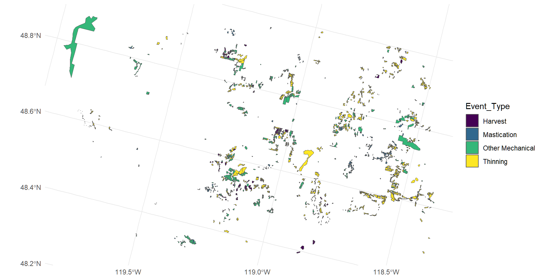
## Clean ----

tx_nonfire <- ready_sf %>%
  # select columns of interest
  select(Event_ID, Year, Event_Type, Event_Subtype, Agency, DB_Source, Start_Date, End_Date) %>%
  # add acres
  mutate(Acres = round(as.numeric(set_units(st_area(.), "acre")), 1)) %>%
  # convert Start_Date and End_Date to date only fields; no time
  mutate(DateStart = ymd(substring(Start_Date, first = 1, last = 10))) %>%
  mutate(DateEnd = ymd(substring(End_Date, first = 1, last = 10))) %>%
  # select final columns
  select(Year, Event_Type)
Explore fire treatments
### FIRE TREATMENTS ----

## Get the data ----

# location of the ready Events example layer
raw_path <- 'inputs\\events_example_data.gdb\\events_raw'

# get the ready data from the gdb
raw_open <- arc.open(path = raw_path)

# select fire treatments for the time period
# list of fire treatment types of interest
fire_types <- c("Prescribed Fire")
# where clause including the year and type of treatments
where_fire <- paste0(
  "Year >= 2004 AND EVENT_TYPE IN ('", paste(fire_types, collapse = "', '"), "')"
  )

# select features using the where clause
raw_select <- arc.select(raw_open, where_clause = where_fire)

# convert the selected data to an sf object
raw_sf <- arc.data2sf(raw_select) %>%
  # make valid
  st_make_valid(raw_sf)

# check it out
ggplot(data = raw_sf) +
  geom_sf(aes(fill = Event_Type)) +
  scale_fill_viridis_d() +
  theme_minimal()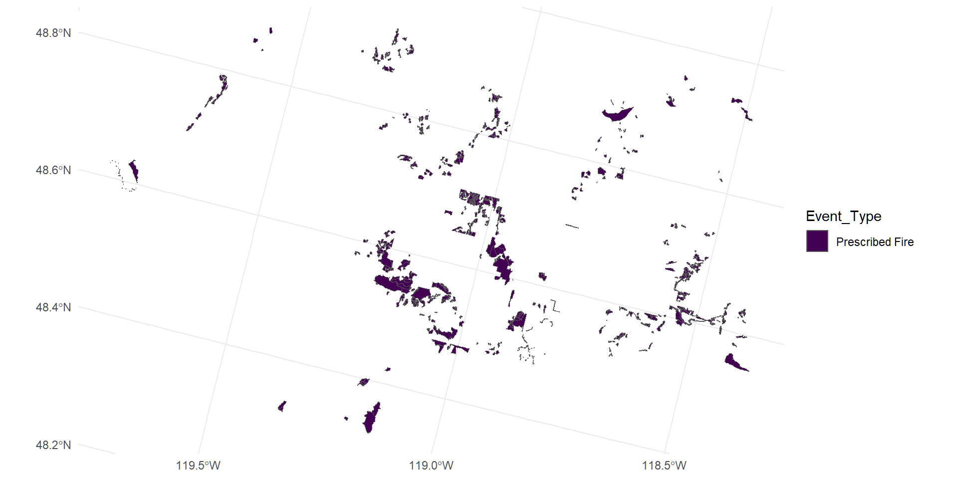
## Clean ----

raw_clean <- raw_sf %>%
  # select columns of interest
  select(Event_ID, Year, Event_Type, Event_Subtype, Agency, DB_Source, Start_Date, End_Date) %>%
  # join the prescribed fire class using the look up table
  left_join(rx_class, by = c("Event_Type", "Event_Subtype")) %>%
  # add acres
  mutate(Acres = round(as.numeric(set_units(st_area(.), "acre")), 1)) %>%
  # convert Start_Date and End_Date to date only fields; no time
  mutate(DateStart = ymd(substring(Start_Date, first = 1, last = 10))) %>%
  mutate(DateEnd = ymd(substring(End_Date, first = 1, last = 10))) %>%
  # remove some columns
  select(-c(Start_Date, End_Date))
Clean overlaps
## Remove overlaps ----

# List of years to process
year_list <- c(2004:2023)

# list of types for final treatment layer
type_list <- c("Burn_broadcast", "Burn_pile", "Burn_unknown")

# prep dataframe for the loops that will remove overlaps below
rawsimple <- raw_clean %>%
  # adjust the treatment type so that includes the class
  mutate(Event_Type = case_when(
    Event_Type == "Prescribed Fire" & Class == "Broadcast" ~ "Burn_broadcast",
    Event_Type == "Prescribed Fire" & Class == "Pile" ~ "Burn_pile",
    Event_Type == "Prescribed Fire" & Class == "Unknown" ~ "Burn_unknown",
    .default = Event_Type)) %>%
  # select columns of interest
  select(Year, Event_Type)

## Remove overlaps, within type ----
# remove overlapping polygons of the same type within the same year
# e.g. 2 pile burns in the same location in the same year

union_polys <- list()

for (year in year_list) {
  for (type in type_list) {

    # filter for year/type combo
    filtered <- rawsimple %>% filter(Year == year, Event_Type == type)

    # union
    union_filtered <- st_union(filtered)

    # check if union_filtered is empty or has a single geometry
    if (length(union_filtered) == 0) {
      next  # skip to the next iteration if no geometries
    }

    # convert the result back to an sf object, add year and type
    # st_union returns a geometry collection, not a full sf object
    union_final <- st_as_sf(data.frame(geometry = union_filtered,
                                       Year = year,
                                       Event_Type = type))

    # store the result in the list
    union_polys[[paste0("y", year, "_", type)]] <- union_final
  }
}

# combine all year/type unioned layers
rawsimple_union <- bind_rows(union_polys)

# explicitly make a valid sf object
rawsimple_union <- st_as_sf(rawsimple_union)
rawsimple_union <- st_make_valid(rawsimple_union)

## Remove overlaps, between types ----
# remove overlapping polygons of different types within the same year
# e.g. a broadcast and a pile burn in the same location in the same year
# When overlpping fire polygons are found in the same year, overlaps are
# removed based on this order of priority: broadcast, pile, unknown. In
# other words, if a broadcast burn overlaps a pile burn in the same year,
# the area of overlap is assigned the type broadcast. When a pile
# burn overlaps an unknown burn in the same year, the area of overlap is
# assigned the type pile.

# Initialize an empty list to store final results
final_results <- list()

for (year in year_list) {

  # filter for each type
  broadcast <- rawsimple_union %>% filter(Year == year, Event_Type == "Burn_broadcast")
  pile <- rawsimple_union %>% filter(Year == year, Event_Type == "Burn_pile")
  unknown <- rawsimple_union %>% filter(Year == year, Event_Type == "Burn_unknown")

  # remove broadcast from piles
  if (nrow(pile) > 0 && nrow(broadcast) > 0) {
    pile_only <- ms_erase(pile, erase = broadcast)
  } else {
    pile_only <- pile
  }
  # combine broadcast and clean piles
  bcast_pile <- rbind(broadcast, pile_only)

  # remove broadcast/pile from unknown
  if (nrow(unknown) > 0 && nrow(bcast_pile) > 0) {
    unknown_only <- ms_erase(unknown, erase = bcast_pile)
  } else {
    unknown_only <- unknown
  }
  # combine broadcast/pile with clean unknown
  bcast_pile_unk <- rbind(broadcast, pile_only, unknown_only)

  # store the result in the list
  final_results[[paste0("final", year)]] <- bcast_pile_unk
}

## Note ----
# a warning is generated here. I'm not sure why and multiple
# attempts to resolve the warning have failed. The results seem OK.

# combine final results for all years
tx_fire <- bind_rows(final_results)

# check it out
ggplot(data = tx_fire) +
  geom_sf(aes(fill = Event_Type)) +
  scale_fill_viridis_d() +
  theme_minimal()
Combine all treatments
### COMBINE ALL TREATMENTS ----

tx_all <- tx_nonfire %>%
  bind_rows(tx_fire)

# check it out
ggplot(data = tx_all) +
  geom_sf(aes(fill = Event_Type)) +
  scale_fill_viridis_d() +
  theme_minimal()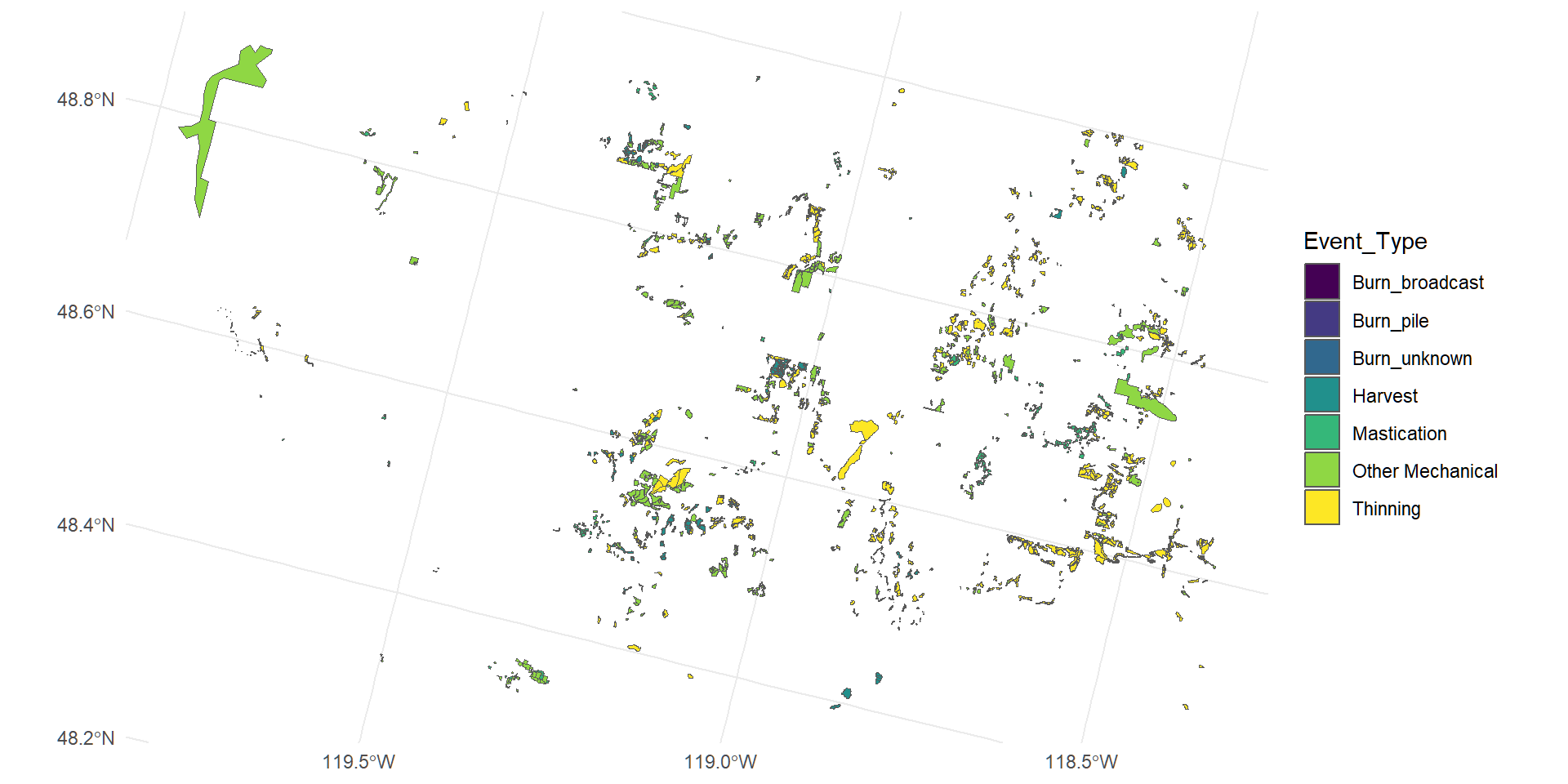
Notes on results
The tx_nonfire layer represents individual treatment polygons.
The tx_fire layer represents the footprint of a given prescribed fire type in a given year. For example, a give year, e.g. 2020, can have up to 3 polygons: one for the footprint for broadcast burns, one for pile, and one for unknown burns. Some years have fewer than three polygons because not all burn types were present in all years. Because the original treatment polygons were unioned, individual treatment units are no longer present in the data.
The tx_nofire layer could be further processed to union polygons by year to produce a layer equivalent to tx_fire.
As processed here, the data are adequate for visualizing and calculating footprint area of non-fire and fire treatments per year.
“Footprint” area is the area of non-overlapping polygons. Overlapping polygons are not present in the Events Ready data used to create tx_nonfire, and I removed overlapping polygons from the Events Raw to produce tx_fire in the code above.
In many areas, treatments overlap between years; e.g., a thin in 2020 followed by a pile burn in 2021. Use transparency to better visualize where multiple entries have occurred.
Users should review documentation on landfire.gov to understand Events data, especially the difference between Events Ready and Events raw.